Building a Real-Time Transport Lakehouse

2M Events · Sub-Minute Latency · Under $1/Month

In September, over just two days, I processed around 2 million real-time events from Helsinki’s public transport system. This made it possible to monitor, with sub-minute latency, how many buses were on the road, what the average delays were, and much more.

---

Real-Time Grafana Dashboard for HSL Transport Data

The same data also powered deeper analysis, from finding the most popular routes to spotting the busiest transport hubs and other key insights.

All of this ran without losing a single event, stayed fully scalable, and, most importantly, running the pipeline for an entire month would cost less than one dollar.

Here’s how I built it.

The Challenge

Helsinki’s public transport system (HSL) publishes a continuous MQTT feed of vehicle events. Thousands of messages flow in every minute:

• Where each bus is right now

• How late or early it is

• Which route it belongs to

Example of a single event produced into Kafka:

{
  “topic”: {
    “prefix”: “hfp”,
    “version”: “v2”,
    “journey_type”: “journey”,
    “temporal_type”: “ongoing”,
    “event_type”: “vp”,
    “transport_mode”: “bus”,
    “operator_id”: “0018”,
    “vehicle_number”: “00947”,
    “route_id”: “6171”,
    “direction_id”: “1”,
    “headsign”: “Kirkkonummi”,
    “start_time”: “12:08”,
    “next_stop”: “2314219”,
    “geohash_level”: “5”,
    “geohash”: “60;24”,
    “sid”: “17”
  },
  “payload”: {
    “VP”: {
      “desi”: “171”,
      “dir”: “1”,
      “oper”: 6,
      “veh”: 947,
      “tst”: “2025-09-11T09:05:32.966Z”,
      “tsi”: 1757581532,
      “spd”: 0.0,
      “hdg”: 274,
      “lat”: 60.159918,
      “long”: 24.73808,
      “acc”: 0.0,
      “dl”: 179,
      “odo”: 0,
      “drst”: 0,
      “oday”: “2025-09-11”,
      “jrn”: 446,
      “line”: 676,
      “start”: “12:08”,
      “loc”: “DR”,
      “stop”: 2314219,
      “route”: “6171”,
      “occu”: 0
    }
  }
}

If you want insights, you need to:

1. Ingest it in real-time

2. Store it reliably

3. Process it into something useful

4. Analyze it interactively

And ideally, you want this system to run on a student budget, able to grow over time without costing more than a few dollars per month.

---

Architecture

The main rationale behind my architecture is the Databricks platform. I see how popular Databricks has become in modern data engineering. Its stack (Spark, Delta Lake, streaming + batch processing, orchestration, notebooks, etc.) covers most real-world scenarios. My goal was to build a simplified, on-premise alternative using open-source tools.

I used a Medallion architecture with three layers:

• Bronze: Raw, untouched data directly from Kafka

• Silver: Cleaned and structured data, prepared for further processing

• Gold: Snowflake-style data model with fact and dimension tables

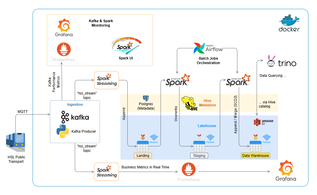
Here’s the stack I chose:

• Kafka for real-time ingestion

• Spark Structured Streaming for processing both real-time and batch data

• Delta Lake on Amazon S3 for storage (ACID transactions, schema evolution)

• Hive Metastore + Trino for SQL queries

• Airflow for orchestrating ETL jobs

• Prometheus + Grafana for real-time metrics

• Docker Compose for easy local deployment

The entire pipeline runs on my laptop plus a tiny S3 bucket. Total cost? Under 5 cents.

---

Making It Real-Time

The real-time processing was the most interesting part.

First, real-time transport data comes in via MQTT (basically a protocol for transferring data from IoT devices) into Kafka:

producer = KafkaProducer(
    bootstrap_servers=’kafka:29092’,
    value_serializer=lambda v: json.dumps(v).encode(’utf-8’),
    key_serializer=lambda k: str(k).encode(’utf-8’)
)

def on_connect(client, userdata, flags, reason_code, properties):
    client.subscribe(”/hfp/v2/journey/#”)

def on_message(client, userdata, msg):

    # ...
    # some custom code to filter messages from MQTT
    # ...

    producer.send(TOPIC, key=kafka_key, value=event_body)

mqttc = mqtt.Client(mqtt.CallbackAPIVersion.VERSION2)
mqttc.on_connect = on_connect
mqttc.on_message = on_message
mqttc.connect(”mqtt.hsl.fi”, 1883, 60)
mqttc.loop_forever()

Spark job listens to Kafka, aggregates events in 5-minute windows (sliding every 30 s), and publishes fresh KPIs to Prometheus every 15 s. Grafana then reads them from Prometheus and updates with sub-minute latency.

Start a tiny HTTP server and define gauges:

from prometheus_client import Gauge, start_http_server
start_http_server(int(os.getenv(”PROM_PORT”, “9108”)))

TOTAL_ACTIVE = Gauge(”total_active_vehicles”, “Active vehicles”)
AVG_SPEED_ALL = Gauge(”avg_speed_all”, “Average speed (km/h)”)
PCT_ON_TIME_1 = Gauge(”pct_routes_on_time_1”, “≤1 min”)
PCT_ON_TIME_2 = Gauge(”pct_routes_on_time_2”, “≤2 min”)
PCT_ON_TIME_3 = Gauge(”pct_routes_on_time_3”, “≤3 min”)

ROUTE_DELAY_EXTREME = Gauge(
    “route_delay_extreme_seconds”,
    “Avg delay extremes in the latest window”,
    [”type”,”route_id”]
)

Read from Kafka and parse only what we need:

kafka_stream = (spark.readStream.format(”kafka”)
    .option(”kafka.bootstrap.servers”,”kafka:29092”)
    .option(”subscribe”,”hsl_stream”)
    .option(”startingOffsets”,”latest”)
    .load())

parsed_df = kafka_stream.selectExpr(”CAST(value AS STRING) AS v”).select(
    F.get_json_object(”v”,”$.topic.route_id”).alias(”route_id”),
    F.get_json_object(”v”,”$.topic.vehicle_number”).alias(”vehicle_number”),
    F.get_json_object(”v”,”$.payload.VP.tst”).alias(”tst”),
    F.get_json_object(”v”,”$.payload.VP.spd”).cast(”double”).alias(”speed”),
    F.get_json_object(”v”,”$.payload.VP.dl”).cast(”double”).alias(”delay”)
).withColumn(”timestamp”, F.to_timestamp(”tst”))

Aggregate in sliding windows with a 1-minute watermark (the watermark could be set much higher if events arrive late, but in this case 1 minute was enough to reduce system and memory load while still keeping processing nearly real-time):

windowed_df = (parsed_df
    .withWatermark(”timestamp”,”1 minutes”)
    .groupBy(F.window(”timestamp”,”5 minutes”,”30 seconds”))
    .agg(
        F.approx_count_distinct(”vehicle_number”).alias(”active_vehicles”),
        F.avg(”speed”).alias(”avg_speed”),
        F.avg(F.when(F.abs(”delay”) <= 60, 1).otherwise(0)).alias(”on_time_1”),
        F.avg(F.when(F.abs(”delay”) <= 120,1).otherwise(0)).alias(”on_time_2”),
        F.avg(F.when(F.abs(”delay”) <= 180,1).otherwise(0)).alias(”on_time_3”),
    )
    .select(F.col(”window.end”).alias(”window_end”),
            “active_vehicles”,”avg_speed”,”on_time_1”,”on_time_2”,”on_time_3”))

Push only the freshest closed window to Prometheus:

def update_prometheus(batch_df, batch_id):
    if batch_df.rdd.isEmpty(): return
    latest_end = batch_df.agg(F.max(”window_end”)).first()[0]
    row = (batch_df.filter(F.col(”window_end”)==latest_end)
                  .limit(1).collect()[0])

    TOTAL_ACTIVE.set(int(row[”active_vehicles”] or 0))
    AVG_SPEED_ALL.set(float(row[”avg_speed”] or 0.0))
    PCT_ON_TIME_1.set(float(row[”on_time_1”] or 0.0))
    PCT_ON_TIME_2.set(float(row[”on_time_2”] or 0.0))
    PCT_ON_TIME_3.set(float(row[”on_time_3”] or 0.0))

Optional route extremes (most delayed and most ahead in the latest window):

route_windowed_df = (parsed_df
    .withWatermark(”timestamp”,”1 minutes”)
    .groupBy(F.window(”timestamp”,”5 minutes”,”30 seconds”), “route_id”)
    .agg(F.avg(”delay”).alias(”avg_delay”), F.count(”*”).alias(”events_cnt”))
    .select(F.col(”window.end”).alias(”window_end”),”route_id”,”avg_delay”,”events_cnt”))

def update_route_extremes(batch_df, batch_id):
    if batch_df.rdd.isEmpty(): return
    latest_end = batch_df.agg(F.max(”window_end”)).first()[0]
    latest = batch_df.filter(F.col(”window_end”)==latest_end).filter(”events_cnt >= 5”)
    if latest.rdd.isEmpty(): return
    ROUTE_DELAY_EXTREME.clear()
    worst = latest.orderBy(F.desc(”avg_delay”)).limit(1).collect()[0]
    best  = latest.orderBy(F.asc(”avg_delay”)).limit(1).collect()[0]
    ROUTE_DELAY_EXTREME.labels(”worst”, worst[”route_id”] or “unknown”).set(float(worst[”avg_delay”] or 0.0))
    ROUTE_DELAY_EXTREME.labels(”best”,  best[”route_id”]  or “unknown”).set(float(best[”avg_delay”] or 0.0))

Start both streams with 15-second triggers and separate checkpoints. Append mode is used so only closed windows are sent to Prometheus, which prevents partial aggregates from appearing and keeps Grafana charts from jumping:

(windowed_df.writeStream.outputMode(”append”)
 .foreachBatch(update_prometheus)
 .option(”checkpointLocation”,”/home/jobs/checkpoint_data/realtime/metrics_totals”)
 .trigger(processingTime=”15 seconds”)
 .start())

(route_windowed_df.writeStream.outputMode(”append”)
 .foreachBatch(update_route_extremes)
 .option(”checkpointLocation”,”/home/jobs/checkpoint_data/realtime/metrics_extremes”)
 .trigger(processingTime=”15 seconds”)
 .start()
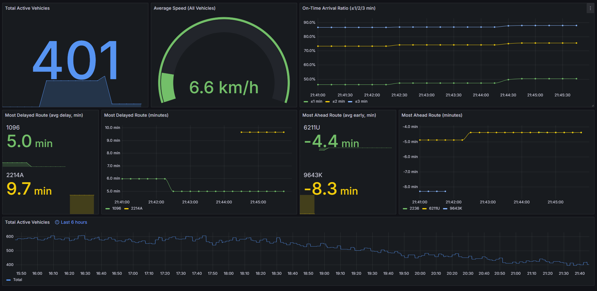
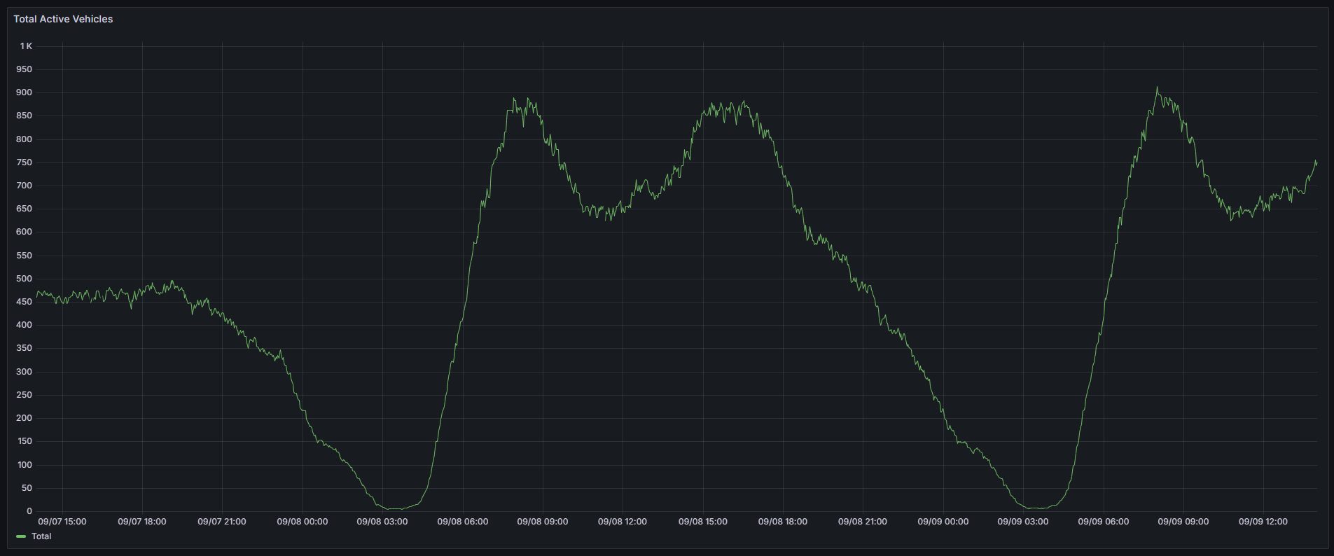
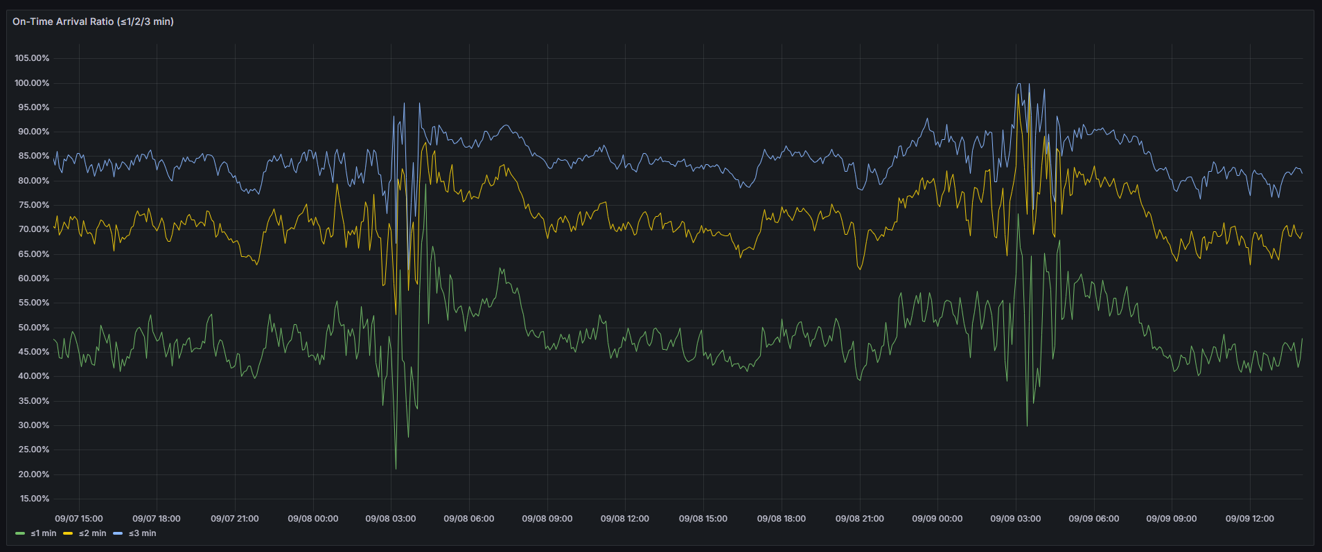
 .awaitTermination())

What you see in Grafana:

Total active vehicles, average speed, on-time ratios (≤1/2/3 min), and the current most delayed and most ahead routes by average delay update in near real time.

---

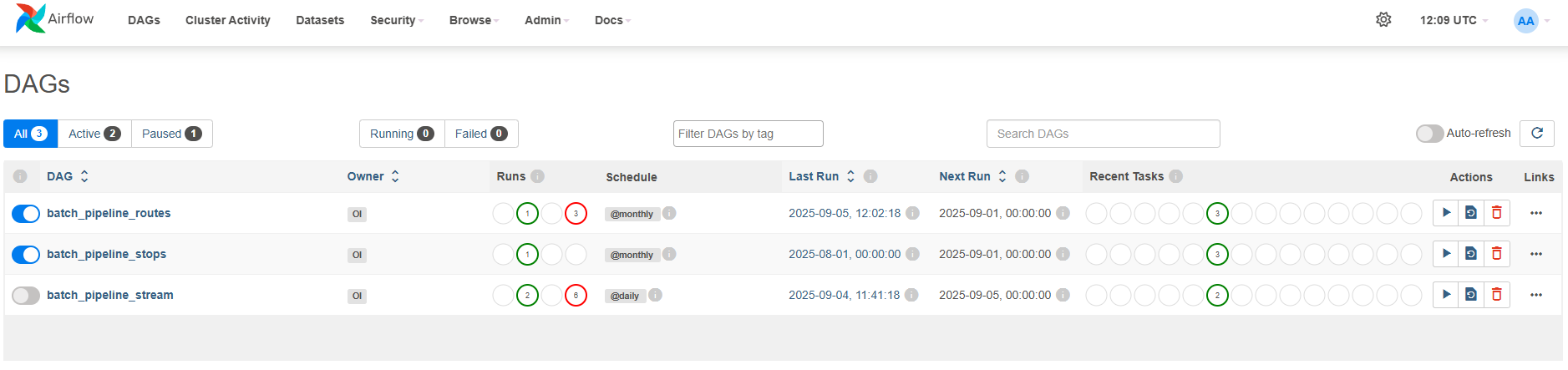
Historical Analytics

For deeper analysis, Airflow triggers batch jobs that transform data into the Gold layer using Slowly Changing Dimensions (SCD2) for routes and stops.

SCD2 without rewriting entire tables:

1. MERGE step marks outdated records as inactive.

    MERGE INTO hdw.dim_routes AS dim
    USING dim_temp AS stg
    ON dim.route_id = stg.route_id
        AND dim.active_flg = 1
        AND (
           dim.route_short_name <> stg.route_short_name OR
           dim.route_long_name <> stg.route_long_name OR
           dim.route_type <> stg.route_type
        )
    WHEN MATCHED THEN UPDATE SET
        dim.effective_end_dt = stg.hist_record_end_timestamp,
        dim.active_flg = stg.hist_record_active_flg,
        dim.update_dt = stg.hist_record_update_dt

2. INSERT step adds new records with updated values.

    INSERT INTO hdw.dim_routes
    SELECT stg.*
    FROM dim_temp stg
    LEFT JOIN hdw.dim_routes dim
        ON stg.route_id = dim.route_id AND dim.active_flg = 1
    WHERE dim.route_id IS NULL

This keeps full history:

• If a bus stop moves or changes name -> the old version is preserved

• If a route gets rebranded -> both old and new versions exist in the data

With Trino + SQL, I could ask questions like:

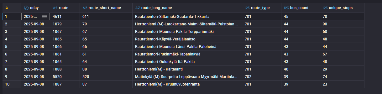
• Which routes are the busiest?

  SELECT 
      f.oday,
      f.route,
      r.route_short_name,
      r.route_long_name,
      r.route_type,
      COUNT(DISTINCT f.vehicle_number) AS bus_count,
      COUNT(DISTINCT f.stop) AS unique_stops,
      ROUND(
          CAST(COUNT(DISTINCT f.vehicle_number) AS DOUBLE) 
          / CAST(COUNT(DISTINCT f.stop) AS DOUBLE),
        2
      ) AS veh_to_stops_ratio
  FROM hdw.fact_vehicle_position f
  JOIN hdw.dim_routes r
      ON f.route_id = r.route_id
      AND r.active_flg = 1
  WHERE f.oday = DATE ‘2025-09-08’
  GROUP BY f.oday, f.route_id, f.route, r.route_short_name, r.route_long_name, r.route_type
  ORDER BY veh_to_stops_ratio DESC
  LIMIT 10;

• Which routes experienced the most delays?

  SELECT 
      f.oday,
      r.route_short_name,
      r.route_long_name,
      ROUND(AVG(f.dl) / 60, 2) AS avg_delay_min
  FROM hdw.fact_vehicle_position f
  JOIN hdw.dim_routes r
      ON f.route_id = r.route_id
      AND r.active_flg = 1
  WHERE f.oday = DATE ‘2025-09-08’
  GROUP BY f.oday, r.route_short_name, r.route_long_name
  ORDER BY avg_delay_min DESC
  LIMIT 10

• Or we can go to the Bronze layer and check for missing events or data loss.

  WITH renamed_t AS (
    SELECT
      partition AS kafka_partition,
      offset AS kafka_offset
    FROM
      hdw_ld.events_ld
  ),
  ordered AS (
    SELECT
      kafka_partition,
      kafka_offset,
      LEAD(kafka_offset) OVER (
        PARTITION BY kafka_partition ORDER BY kafka_offset
      ) AS next_offset
    FROM
      renamed_t
  ),
  gaps AS (
    SELECT
      kafka_partition,
      kafka_offset + 1 AS missing_start,
      next_offset - 1 AS missing_end,
      (next_offset - kafka_offset - 1) AS missing_count
    FROM
      ordered
    WHERE
      next_offset IS NOT NULL
      AND next_offset > kafka_offset + 1
  )
  SELECT
    *
  FROM
    gaps;

---

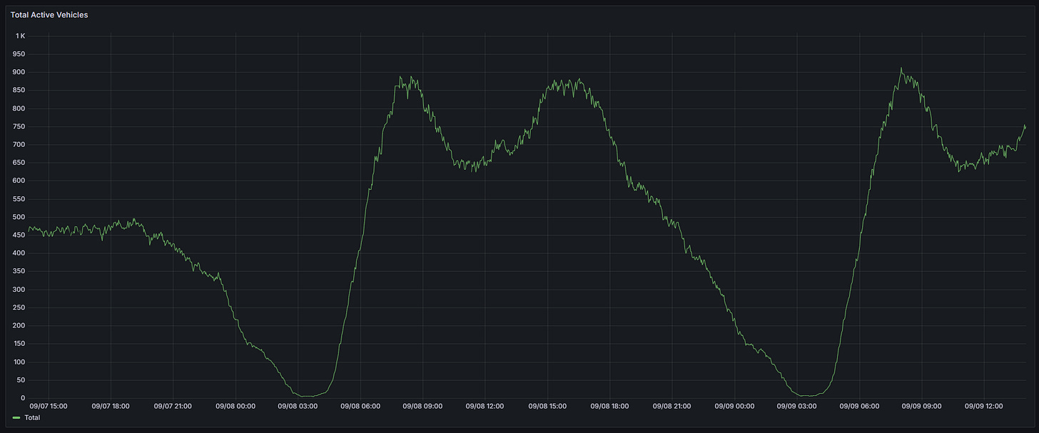
Favorite Insights (2 days time window)

• Peak traffic: 7–9 AM and 3–6 PM with ~890 buses simultaneously on the road

  

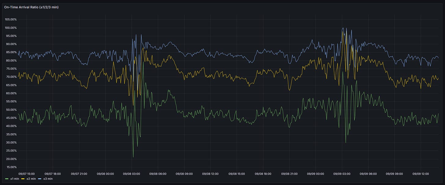
• On-time arrival performance:

  • Within 3 min: About 80–85% of buses arrive on time

  • Within 2 min: Around 70–75% stay within two minutes of schedule

  • Within 1 min: About 40–50% manage to stay within one minute

    

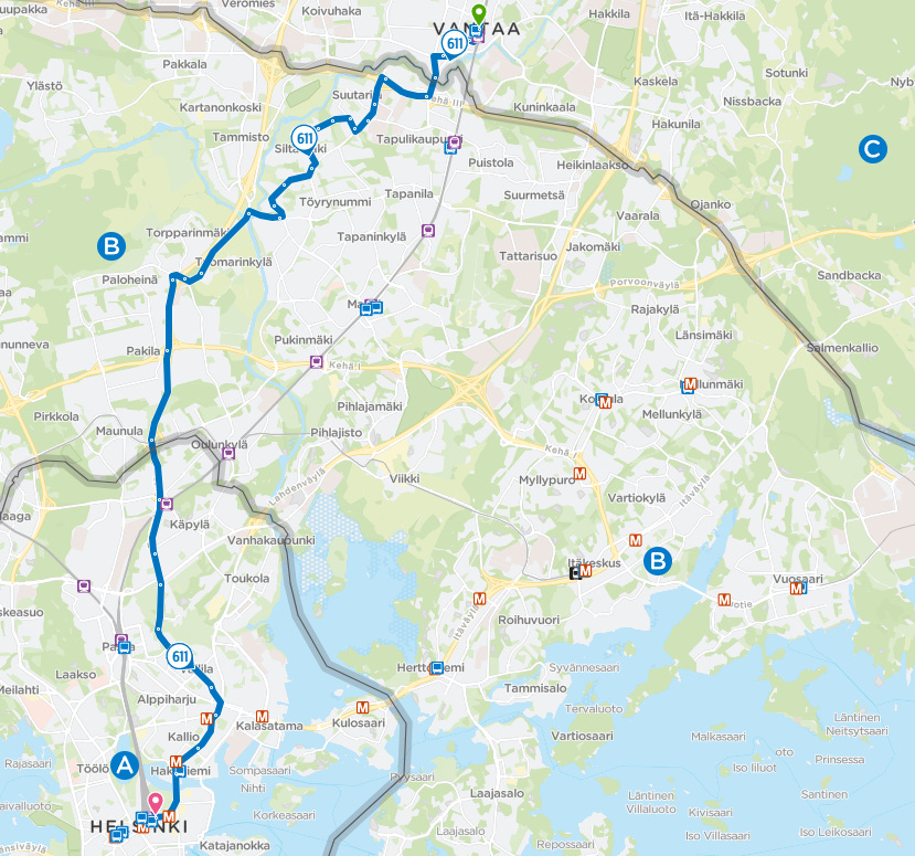
• Most operationally intensive: Route 611 with 45 buses in one day

  

  

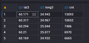
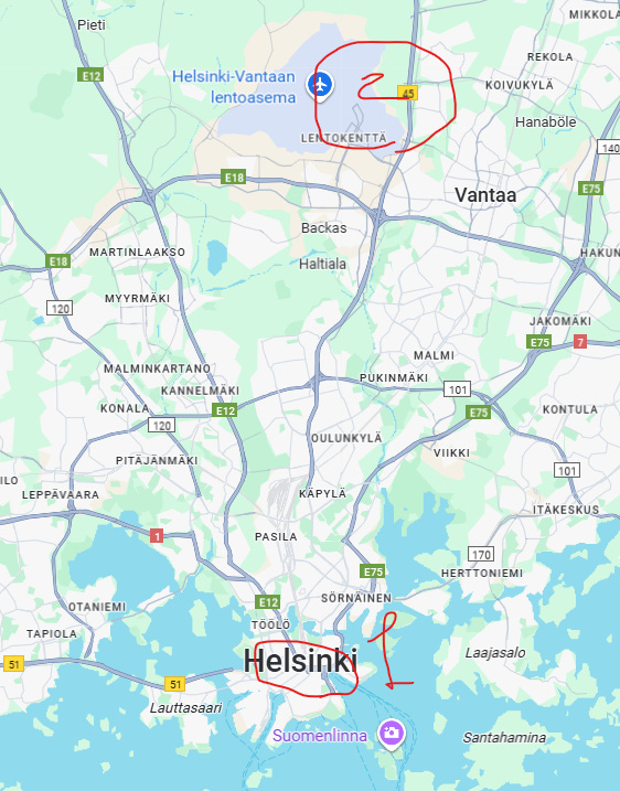
• Biggest stop hub (no surprise here): Helsinki Central Railway Station

  

  

I also discovered Route 99V had an unusually high veh_to_stops ratio (how many distinct vehicles served a route compared to the number of unique stops that day).

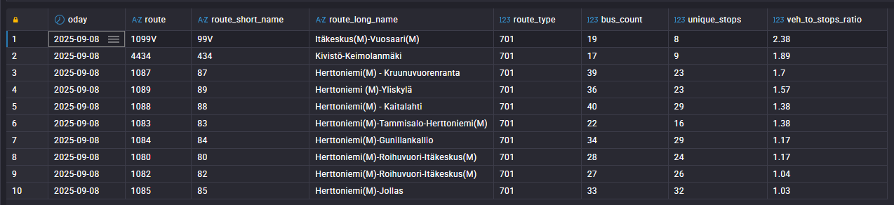
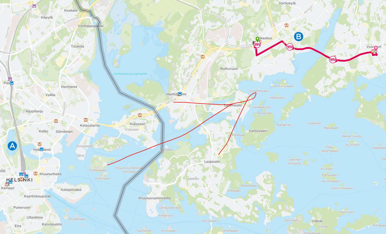
After doing some research it turned out that this bus is actually a metro replacement service between Itäkeskus–Rastila–Vuosaari, added due to the temporary suspension of Metro service to Vuosaari and Rastila during the bridge renovation. The line ran as frequently as every 2.5 minutes at peak, which explains the high bus-to-stops density on that date.

Source: https://www.hsl.fi/en/hsl/news/service-updates/2025/03/no-metro-services-to-vuosaari-or-rastila-from-5-may--we-will-increase-bus-services-in-the-area

---

Where It Can Be Applied

While this project is demonstrated using public transport data, the underlying streaming Lakehouse design is applicable to a wide range of industries, particularly those that need to process millions of events per day in a cost-effective, open-source environment:

• Startups and mid-sized businesses – building scalable products without committing to expensive managed platforms.

• IoT and mobility – processing millions of device and vehicle events per day in real time.

• Gaming companies – tracking player telemetry, in-game transactions, and live events at scale.

• Financial services and fintech – streaming transactions, fraud detection, and real-time risk monitoring on high-volume event streams.

• Telecom and streaming providers – handling continuous event streams such as usage data, sessions, or content delivery metrics.

---

Taking the Project Further

For anyone looking to build on top of this pipeline, the most valuable additions would be:

• Adding trams, metro, and trains to increase coverage.

• Adding a simple Kafka connector to save incoming events as raw files and then load the landing layer from these files instead of directly from the Kafka topic. This provides an additional way to store and replay data if needed.

• Deploying on Kubernetes to scale Spark nodes for larger workloads.

---

Final Thoughts

Building this project was like watching a city breathe in real time. At one moment, you see the busy rush hour; at the next, the quiet of 3 AM with only a few buses running.

And the best part? Everything runs on open-source tools, a bit of cloud storage, and a lot of curiosity.

---

References

1. Project GitHub repo

2. HSL Open Data

3. GTFS Overview

4. Extended route types

---

Community

This article is written by Oleg Ivantsov for an open source community called DataTribe Collective.